

Regression analysis in Excel measures how one number changes when another number changes, such as how test scores move with hours studied. Excel offers two methods: the Analysis ToolPak, a built-in add-in that produces a full statistics report automatically, and regression functions like SLOPE, LINEST, and FORECAST.LINEAR, which each return one result in a cell.
This guide covers both methods, a step-by-step walkthrough with a sample dataset, how to read the output, the core functions, how to add a regression line to a chart, and common errors with their fixes.
Excel is one of the most prominent tools that is widely used, but there are other statistics software for students that you will benefit from.
Your data’s ready, but the paper is not
The deadline won’t move, so let a writer take the research paper off your plate now.

What is regression analysis in Excel?
Regression analysis in Excel is a statistical method that fits a line or curve to a set of data points to describe the relationship between two variables. The result is an equation that predicts one value (y) from another (x), most often the straight line y = mx + b.
In the equation y = mx + b, each part means:
- y is the predicted value (the outcome being estimated)
- x is the known input (the value used to make the prediction)
- m is the slope (how much y changes for each one-unit rise in x)
- b is the intercept (the value of y when x equals 0)
Linear regression analysis in Excel fits this straight line, known as the least squares regression line because it keeps the total gap between the data points and the line as small as possible, and suits data that climbs or falls at a steady rate. Exponential regression fits the curve y = b*m^x instead, which suits data that grows by a percentage each step, such as compound interest or population growth. Excel handles linear models with SLOPE, LINEST, and TREND, and exponential models with LOGEST and GROWTH.
How to do a regression analysis in excel?
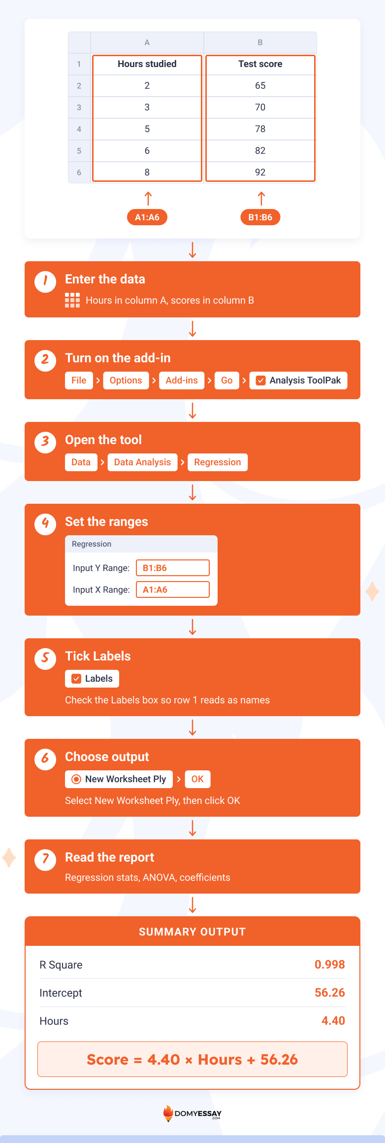
How to run regression in Excel comes down to one tool: the Analysis ToolPak. Enable it, open Data > Data Analysis > Regression, set the Y and X ranges, and click OK. Excel then builds a full summary report on a new sheet. The sample below uses 5 students’ study hours and test scores.
- Enter the data. Put hours studied in column A (A1 as the header, A2:A6 for values) and test scores in column B (B1 header, B2:B6 values).
- Turn on the add-in. Go to File > Options > Add-ins, pick Excel Add-ins next to Manage, click Go, check the Analysis ToolPak box, and click OK.
- Open the tool. On the Data tab, click Data Analysis, select Regression, and click OK.
- Set the ranges. In Input Y Range, select B1:B6 (the scores). In Input X Range, select A1:A6 (the hours).
- Tick Labels. Because row 1 holds headers, check the Labels box so Excel reads them as names, not data.
- Choose output. Select New Worksheet Ply, then click OK.
- Read the report. Excel creates a sheet with Regression Statistics, ANOVA, and a coefficients table.
If you need a solid topic to write about, choose something from our list of statistics project ideas.
How to read the regression output?
The regression output reports four key numbers. R Square shows how well the line fits (0 to 1). Significance F shows whether the model is statistically meaningful. The coefficients give the equation. The p-values show whether each variable matters. For the sample data, R Square is 0.998.
Significance F and the p-values both come from hypothesis testing, the method that checks whether a relationship is statistically real or down to chance.
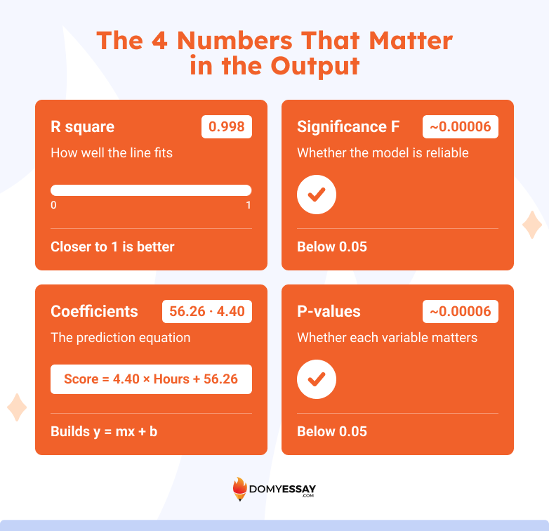
R Square (the coefficient of determination) measures the share of variation in Y that X explains. The sample value of 0.998 means study hours account for 99.8% of the variation in test scores, a strong fit. Values near 1 indicate a tight fit, and values near 0 indicate a weak one.
Significance F tests whether the overall model is reliable. A value below 0.05 means the relationship is statistically meaningful. The sample model returns a Significance F well below 0.05 (roughly 0.00006 for this dataset).
Coefficients build the prediction equation. The Intercept coefficient is 56.26, and the Hours coefficient (the slope) is 4.40. That produces the equation score = 4.40 × hours + 56.26, so each extra hour of study predicts about 4.4 more points.
P-values test each coefficient separately. A p-value under 0.05 means that variable has a statistically significant effect. The slope’s p-value for the sample data is about 0.00006, well under 0.05, which confirms hours studied is a meaningful predictor of score.
Excel regression functions
Excel regression functions return specific regression results in a single cell without the full ToolPak report. Nine functions cover the common needs: SLOPE, INTERCEPT, RSQ, FORECAST.LINEAR, TREND, LINEST, STEYX, LOGEST, and GROWTH. The table below maps each function to what it returns.
SLOPE, INTERCEPT, and RSQ
SLOPE, INTERCEPT, and RSQ return the three core pieces of a linear regression: the slope, the intercept, and the fit quality. Each takes the known Y values first and the known X values second. For the sample study data, they return 4.40, 56.26, and 0.998.
- SLOPE returns m, the rate of change. =SLOPE(B2:B6, A2:A6) returns 4.40, meaning the score rises 4.40 points per study hour.
- INTERCEPT returns b, the value of Y when X is 0. =INTERCEPT(B2:B6, A2:A6) returns 56.26, the predicted score for 0 hours of study.
- RSQ returns R squared, the fit quality from 0 to 1. =RSQ(B2:B6, A2:A6) returns 0.998, meaning the line explains 99.8% of the variation in scores.
Together these three results build and grade the equation score = 4.40 × hours + 56.26. SLOPE and INTERCEPT define the line, and RSQ confirms how closely the data follows it.
FORECAST.LINEAR and TREND
FORECAST.LINEAR and TREND both predict Y values from the fitted line, but FORECAST.LINEAR returns one prediction while TREND returns several. For the sample data, predicting a 7-hour student gives a score of about 87.1 from either function.
- FORECAST.LINEAR predicts a single Y for one new X. Its syntax puts the new X first: =FORECAST.LINEAR(7, B2:B6, A2:A6) returns about 87.1, the predicted score for 7 study hours. Use it when one forecast in one cell is enough.
- TREND predicts Y values for one or many new X values along the same line. Its syntax is =TREND(known_ys, [known_xs], [new_xs], [const]). Entering =TREND(B2:B6, A2:A6, 7) also returns about 87.1, and feeding a range of new X values returns a matching list of predictions. In Microsoft 365, TREND spills the results down automatically; in older versions, select the output range first and press Ctrl+Shift+Enter.
The main difference is volume. FORECAST.LINEAR answers one question at a time, while TREND forecasts a whole column of future values at once. Both rely on the same least-squares line, so a single X produces the same result in either function.
LINEST and STEYX
LINEST and STEYX return deeper regression statistics than the single-value functions. LINEST reports the slope, intercept, and fit measures in one array, while STEYX reports how far the data typically falls from the line. For the sample data, STEYX returns 0.60.
LINEST is the most complete regression function in Excel. Its syntax is =LINEST(known_ys, [known_xs], [const], [stats]). Setting the fourth argument to TRUE returns a full statistics block. For the sample, =LINEST(B2:B6, A2:A6, TRUE, TRUE) returns the slope 4.40 and intercept 56.26 in the top row, with standard errors, R squared (0.998), the F statistic, and the sums of squares in the rows below. Searching for linest excel usually points here, because this one function replaces several separate formulas.
In Microsoft 365, type the formula in one cell and press Enter, and the results spill across a 2-column, 5-row block. In Excel 2019 and earlier, select that block first, then press Ctrl+Shift+Enter to enter it as an array.
STEYX returns the standard error of the estimate, the typical gap between the actual Y values and the values the line predicts. Its syntax is =STEYX(known_ys, known_xs). For the sample, =STEYX(B2:B6, A2:A6) returns 0.60, meaning predicted scores land within roughly 0.6 points of the real scores on average. A smaller STEYX signals a tighter, more accurate fit.
LOGEST and GROWTH
LOGEST and GROWTH handle exponential regression, the curve y = b*m^x, for data that grows by a percentage each step. LOGEST returns the curve’s coefficients, and GROWTH returns predicted values along the curve. For values that double each period, GROWTH predicts the next point as 64.
- LOGEST fits an exponential curve and returns its coefficients. Its syntax is =LOGEST(known_ys, [known_xs], [const], [stats]). For Y values 2, 4, 8, 16, 32 against X values 1 to 5, LOGEST returns m = 2 and b = 1, meaning each step doubles the value.
- GROWTH predicts Y values on that exponential curve. Its syntax is =GROWTH(known_ys, [known_xs], [new_xs]). Using the same doubling data with a new X of 6 returns 64, the next value in the sequence. Use LOGEST and GROWTH only when data curves upward at an accelerating rate; for steady, straight-line change, the linear functions give a better fit.
How to add a regression line to a chart?
To add a regression line to a chart, create a scatter chart from the data, right-click any data point, choose Add Trendline, pick Linear, then tick Display Equation on chart and Display R-squared value on chart. Excel draws the best-fit line with its equation.
- Select the data. Highlight both columns, including the headers (A1:B6 in the sample).
- Insert a scatter chart. On the Insert tab, click the Scatter (X Y) chart icon and choose the first plain scatter option.
- Open trendline options. Right-click any plotted point and select Add Trendline.
- Choose Linear. In the Format Trendline panel, select Linear for a straight-line fit, or Exponential for a curve.
- Show the equation and R². Check Display Equation on chart and Display R-squared value on chart. The line now shows y = 4.40x + 56.26 and R² = 0.998.

See some excel formatting tips while you’re at it.
Common errors in regression analysis and how to fix them
Most regression analysis errors in Excel come from how the data is selected or arranged, not from the math. The four problems below cover the common failures, each with its cause and fix.
- No Data Analysis button. Cause: the Analysis ToolPak is not loaded. Fix: go to File > Options > Add-ins > Go, and check Analysis ToolPak.
- #REF! or wrong coefficients. Cause: the X and Y ranges overlap or are swapped. Fix: select separate, equal-length ranges, with Y as the outcome and X as the predictor.
- #N/A error in a function. Cause: the X and Y ranges have different lengths. Fix: make both ranges cover the same number of rows.
- Labels read as data. Cause: headers were included without ticking Labels. Fix: check the Labels box, or exclude the header row from the range.
If all of this sounds like too much to handle for you, you can always ask us, ‘Do my Excel homework for me.’
Essay’s due?
Don’t let the clock win. Instead, let a writer finish the paper while you sleep.

Final thoughts
Regression analysis in Excel comes down to two paths: the Analysis ToolPak for a full statistics report, and functions like SLOPE, LINEST, FORECAST.LINEAR, and GROWTH for single results. Linear models fit straight-line data, and exponential models fit percentage growth. A scatter chart with a trendline turns the same relationship into a clear visual with its equation and R-squared value.